When someone thinks sexy science, a statistical method doesn’t usually come to mind. However, Nate Silver — a baseball statistician who made a name for himself by analyzing political polls for more than four years — made people who usually shun such topics aware of a technique known as Bayesian inference. Silver used Bayesian methods to combine the results of various polls, analyze them, and predict the probability of a given candidate winning the majority of votes in a district. In each race (presidential and senatorial) in the 2012 election in the United States, the candidate he listed as most likely to win did.

The key to Silver’s success was twofold. He assumed (shockingly enough) that political polls in general are largely accurate, based on the outcomes of previous elections, though some individual polling agencies may be more biased than others. Second, he used each successive poll to refine his predictions of how the election was likely to go — a method from Bayesian inference that lets prior knowledge help predict the likelihood of future outcomes. Since there are many political polls, but not that many elections, Silver’s approach was very sensible.

Bayesian methods are named for the Reverend Thomas Bayes, an 18th century English Presbyterian minister and amateur mathematician who was interested toward the end of his life in probability theory. People dispute over whether Bayes was the first to write down the theorem bearing his name, and it’s certainly true that Bayesian inference goes far beyond what the good reverend wrote.

Bayes’ paper on probability was published in 1763 after his death. In honor of the 250th anniversary of its appearance, Science published a piece about Bayes’ theorem and why it’s a fairly controversial piece of math. I covered that story for Ars Technica:

Bayes’ theorem in essence states that the probability of a given hypothesis depends both on the current data and prior knowledge. In the case of the 2012 United States election, Silver used successive polls from various sources as priors to refine his probability estimates. (In other words, saying he “predicted” the outcome of the election is slightly misleading: he calculated which candidate was most likely to win in each state based on the polling data.) In other cases, priors could be the outcome of earlier experiments or even educated assumptions drawn from experience. The wise statistician or scientist constructs priors that are informative, but that isn’t always easy to do. [Read more…]

I’ve used Bayesian methods and their major competitor, “frequentist” statistics, so like many people I’m somewhat pragmatic about it. (You can definitely find zealots on both “sides” of the issue, though. I will laugh at you if you bring that into my comments, though.) As with many techniques, Bayesian methods work best when they aren’t applied blindly, and it may be more possible to misapply Bayes’ theorem than other statistical techniques.

A simple Bayesian tutorial

So, how does Bayes’ theorem work? The key is comparing existing data to a hypothesis: what is the probability of this outcome if a given hypothesis is true? The theorem uses prior knowledge — itself stated as a probability — to modify the likelihood, so under ideal circumstances the method is very efficient. Under less than ideal circumstances, the priors aren’t very well motivated, and can lead to … nonsense. Let’s say nonsense.

Here’s the theorem in mathematical form: 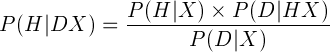 (This way of writing Bayes’ theorem is due to the eccentric physicist E. T. Jaynes.) The P stands for “probability”, H is the hypothesis we’re testing, D is our data, and X is any prior information we might have. In a given situation, we have the data already. Each piece of the equation is a phrase: P (A | B ) reads “the probability of A happening, assuming B. In summary, then:

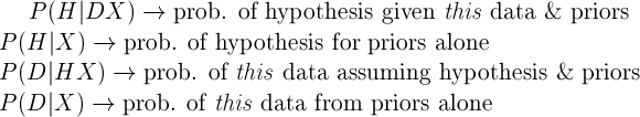
All of these probabilities are numbers between 0 and 1, with 0 meaning “not a chance” and 1 meaning “definitely”. So, Bayes’ theorem reads: the probability of a hypothesis being true (based on the data and prior information) depends on the probability of the hypothesis from prior knowledge, multiplied by the likelihood of that particular data showing up, divided by the chance of the data showing up based on the priors alone.

Using Bradley Efron’s example from his Science article, consider the case of a couple whose sonogram showed they were due to give birth to male twins. Given that data, they wanted to know what the chances were that the twins would be identical as opposed to fraternal — a genetic question undecidable by sonogram. (All of these numbers are reasonable estimates rather than truly accurate values, but it’s good enough for a tutorial.)

One-third of all twins are identical, so  However, half of all pairs of twins are the same sex, meaning that

The final prior is harder: what is the probability of getting a pair of twin boys out of all possible twin combinations? That combines two possibilities — the odds of the twins being fraternal, and the odds of the twins being identical — and excludes any pairing where one twin is a girl.   As we already saw, half of identical twins are boys and one-third of all twins are identical, so  On the other hand, only one-quarter of all fraternal twin pairings will be two boys (think of the odds of flipping two coins and coming up with two tails), and fraternal twins represent the other two-thirds of all twins born: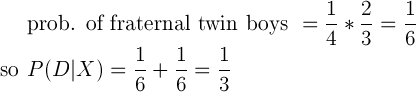

Putting it all together, we find that the odds of having identical twin boys given sonogram data showing two boys is 50 percent: 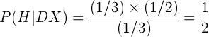 That seems like a lot of work to get equal odds, but a naive assessment of the probability — not including the priors — would seem to indicate only 33 percent chance. As it turns out, the Bayesian treatment gets the right answer.